A tutorial about drawing Sankey graphics using matplotlib
In this post, we'll write a quick Sankey diagram tutorial using the matplotlib tools for that.
What are Sankey diagrams?
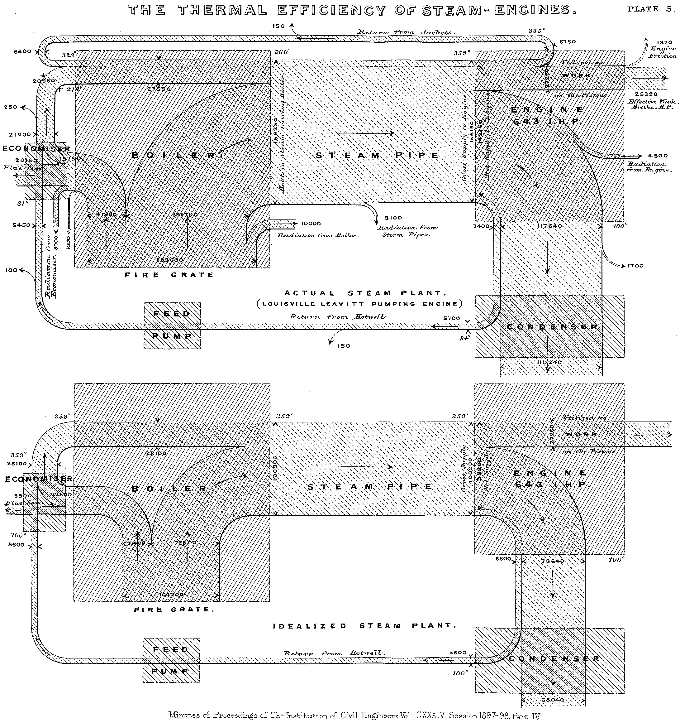
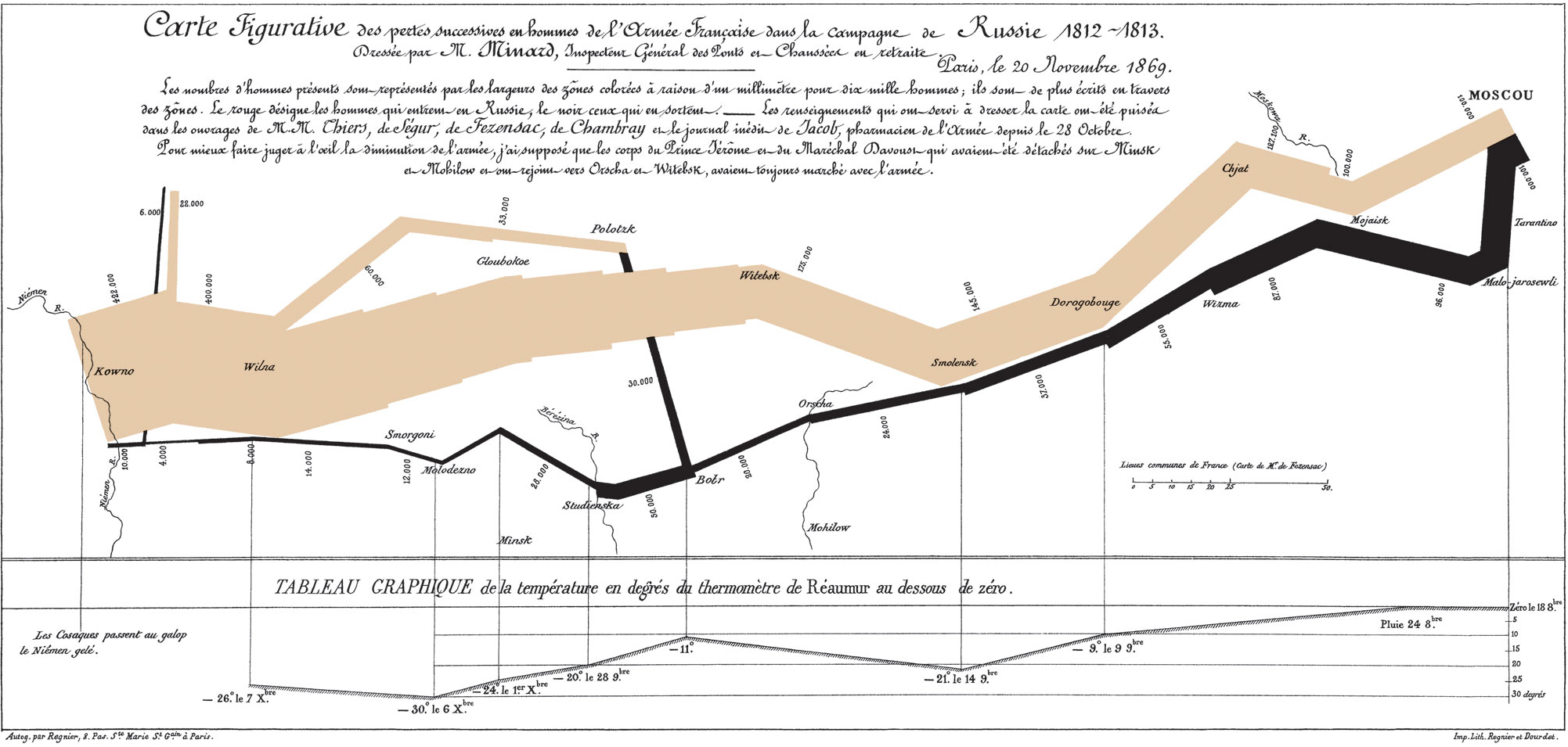
Sankey diagrams are diagrams representing flows between different nodes by using arrows whose width scales according to the value of the flow.
Two of the most famous Sankey diagrams (named after Irish captain Sankey) are Sankey's steam engine efficiency diagram and Minard's map of the French losses during the 1812 Russian campaign.


As one can see in the diagrams above, Sankey diagrams have the following components:
- individual "systems" or boxes (think of the steam engine components)
- that have inputs and outputs
- these inputs and outputs can be represented as branches that align with the system (they can flow from left, right or parallel to the system)
- the boxes connect to each other
These diagrams can be quite complicated to draw. Luckily for us, the matplotlib package comes with ways to draw these diagrams easily. Unfortunately, the documentation is not so easy to understand. That's where this tutorial comes in.
How do Sankey diagrams work within matplotlib?
It turns out that matplotlib comes with a module named matplotlib.sankey. Its API documentation is here.
Also, the following examples are available :
- a basic example, with a simple system and two connected systems
- an example with links between systems
- a complex example drawing the Rankine cycle
Generally, a Sankey diagram ought to be built like this:
sankey = Sankey()
sankey.add() # 1
sankey.add() # 2
#...
sankey.add() # n
sankey.finish()
Alternatively, one can do something like this:
Sankey().add().add... .add().finish()
This being said, let's move to our first diagram.
Our first Sankey diagrams
In this section, we first import the necessary matplotlib tools.
# import matplotlib
%matplotlib inline
import matplotlib.pyplot as plt
from matplotlib.sankey import Sankey
We now build a Sankey with an input flow and an output flow of 1. The flows are specified with the flows argument, while labels are provided using labels.
sankey = Sankey()
sankey.add(flows=[1, -1],
       labels=['input', 'output'])
sankey.finish()
[Bunch(angles=[0, 0], flows=[ 1 -1], tips=[[ 0.16954982  0.        ]
  [ 0.6947228   0.        ]], texts=[<matplotlib.text.Text object at 0x10ed4dc50>, <matplotlib.text.Text object at 0x10ed57128>], patch=Poly((-0.25, 0.5) ...), text=Text(0,0,''))]
There are other arguments that can be specified. For instance, one can change the orientation of the diagram using the rotation argument:
sankey = Sankey()
sankey.add(flows=[1, -1],
       labels=['input', 'output'],
          rotation=-90)
sankey.finish()
[Bunch(angles=[-1.0, -1.0], flows=[ 1 -1], tips=[[  1.03819319e-17  -1.69549816e-01]
  [  4.25395029e-17  -6.94722805e-01]], texts=[<matplotlib.text.Text object at 0x10f048b38>, <matplotlib.text.Text object at 0x10f048fd0>], patch=Poly((0.5, 0.25) ...), text=Text(0,0,''))]
Let's go a step further by providing a third flow to our diagram. To do this, we need to specify an orientations argument. In the previous diagram, we had only to flows, so by default the Sankey module assumes those to be input and output. Now, we need to specify how the flows align with the diagram using a list of orientations. Here, putting an orientation of 1 means it comes from the side.
sankey = Sankey()
sankey.add(flows=[1, -1, 0.5],
           orientations=[0, 0, 1],
           labels=['input', 'output', 'third flow (input)'],
           rotation=-90)
sankey.finish()
[Bunch(angles=[-1.0, -1.0, 2.0], flows=[ 1.  -1.   0.5], tips=[[ -2.50000000e-01   5.80450184e-01]
  [  4.25395029e-17  -6.94722805e-01]
  [  7.90225092e-01   7.50000000e-01]], texts=[<matplotlib.text.Text object at 0x10f0f6f98>, <matplotlib.text.Text object at 0x10f0fe400>, <matplotlib.text.Text object at 0x10f0fe978>], patch=Poly((0.75, 0.25) ...), text=Text(0,0,''))]
The same thing can be done for an output (a fourth flow), but on the other side:
sankey = Sankey()
sankey.add(flows=[1, -1, 0.5, -0.5],
           orientations=[0, 0, 1, -1],
           labels=['input', 'output', 'third flow (input)', 'fourth flow (output)'],
           rotation=-90)
sankey.finish()
[Bunch(angles=[-1.0, -1.0, 2.0, 2.0], flows=[ 1.  -1.   0.5 -0.5], tips=[[-0.25        0.58045018]
  [ 0.25       -1.4447228 ]
  [ 0.79022509  0.75      ]
  [-1.2349479  -0.75      ]], texts=[<matplotlib.text.Text object at 0x10f1b06d8>, <matplotlib.text.Text object at 0x10f1b0b70>, <matplotlib.text.Text object at 0x10f1b5128>, <matplotlib.text.Text object at 0x10f1b50f0>], patch=Poly((0.75, 0.25) ...), text=Text(0,0,''))]
This is fun and all, but let's now see how we can connect two diagrams together.
Connecting diagrams together
The API documentation states that to connect sankey diagrams together, we need to provide the following arguments:
priorwhich is an index of the prior diagram to which this diagram should be connectedconnectwhich is a(prior, this)tuple indexing the flow of the prior diagram and the flow of this diagram which should be connected
Basically prior is the zero based index of the previous diagram element. connect however is more cryptic. Let's start again with a simple input output diagram and try to connect it to another one.
sankey = Sankey()

# first diagram, indexed by prior=0
sankey.add(flows=[1, -1],
       labels=['input', 'output'])

# second diagram indexed by prior=1
sankey.add(flows=[1, -1],
          labels=['input2', 'output2'],
          prior=0,
          connect=(1, 0))
sankey.finish()
[Bunch(angles=[0, 0], flows=[ 1 -1], tips=[[ 0.16954982  0.        ]
  [ 0.6947228   0.        ]], texts=[<matplotlib.text.Text object at 0x10f381400>, <matplotlib.text.Text object at 0x10f381898>], patch=Poly((-0.25, 0.5) ...), text=Text(0,0,'')),
 Bunch(angles=[0, 0], flows=[ 1 -1], tips=[[ 0.6947228   0.        ]
  [ 1.21989579  0.        ]], texts=[<matplotlib.text.Text object at 0x10f387be0>, <matplotlib.text.Text object at 0x10f38d0b8>], patch=Poly((0.275173, 0.5) ...), text=Text(0.525173,0,''))]
It turns out that we can now give a simpler explanation of the connect argument: it says which flows (indexed in the order they were defined) should be connected. So connect should really be described as
connect = (index_of_prior_flow, index_of_current_diagram_flow) that need to be connected
As one can see, the previous diagram does not look very nice. We can correct that by specifying the trunk lengths for each diagram (make them shorter or longer). According to the API:
trunklength: length between the bases of the input and output groups
sankey = Sankey()
# first diagram, indexed by prior=0
sankey.add(flows=[1, -1],
       labels=['input', 'output'],
          trunklength=3)
sankey.add(flows=[1, -1],
          labels=['input2', 'output2'],
           trunklength=1.0,
          prior=0,
          connect=(1, 0))
sankey.finish()
[Bunch(angles=[0, 0], flows=[ 1 -1], tips=[[-0.83045018  0.        ]
  [ 1.6947228   0.        ]], texts=[<matplotlib.text.Text object at 0x10f56d390>, <matplotlib.text.Text object at 0x10f56d828>], patch=Poly((-1.25, 0.5) ...), text=Text(0,0,'')),
 Bunch(angles=[0, 0], flows=[ 1 -1], tips=[[ 1.6947228   0.        ]
  [ 2.21989579  0.        ]], texts=[<matplotlib.text.Text object at 0x10f573b00>, <matplotlib.text.Text object at 0x10f573f98>], patch=Poly((1.27517, 0.5) ...), text=Text(1.52517,0,''))]
Another argument that can be used is the pathlength. These only work for top and bottom flows. Again, according to the API:
list of lengths of the arrows before break-in or after break-away If a single value is given, then it will be applied to the first (inside) paths on the top and bottom, and the length of all other arrows will be justified accordingly. The pathlengths are not applied to the horizontal inputs and outputs.
We can make another example for them:
sankey = Sankey()
# first diagram, indexed by prior=0
sankey.add(flows=[1, -1, 0.1, 0.3],
           orientations=[0, 0, 1, -1],
       labels=['input', 'output', 'top', 'bottom'],
          pathlengths=[0, 0, 0.5, 1.0])
sankey.add(flows=[1, -1],
           labels=['input2', 'output2'],
           trunklength=3.0,
          prior=0,
          connect=(1, 0))
sankey.finish()
[Bunch(angles=[0, 0, 3, 1], flows=[ 1.  -1.   0.1  0.3], tips=[[-0.38045018  0.1       ]
  [ 0.6947228   0.        ]
  [-0.55        1.15804502]
  [-0.65       -1.57413506]], texts=[<matplotlib.text.Text object at 0x10f623a90>, <matplotlib.text.Text object at 0x10f623eb8>, <matplotlib.text.Text object at 0x10f6284a8>, <matplotlib.text.Text object at 0x10f628438>], patch=Poly((-0.25, 0.7) ...), text=Text(0,0,'')),
 Bunch(angles=[0, 0], flows=[ 1 -1], tips=[[ 0.6947228   0.        ]
  [ 3.21989579  0.        ]], texts=[<matplotlib.text.Text object at 0x10f630cf8>, <matplotlib.text.Text object at 0x10f6341d0>], patch=Poly((0.275173, 0.5) ...), text=Text(1.52517,0,''))]
Now that we understand the basics, we can also build a diagram that introduces that outputs the second system to the bottom (by using an orientation of -1).
sankey = Sankey()
# first diagram, indexed by prior=0
sankey.add(flows=[1, -1, 0.1, 0.3],
           orientations=[0, 0, 1, -1],
       labels=['input', 'output', 'top', 'bottom'],
          pathlengths=[0, 0, 0.5, 1.0])
sankey.add(flows=[1, -1],
           orientations=[0, -1],
           labels=['input2', 'output2'],
           trunklength=3.0,
          prior=0,
          connect=(1, 0))
sankey.finish()
[Bunch(angles=[0, 0, 3, 1], flows=[ 1.  -1.   0.1  0.3], tips=[[-0.38045018  0.1       ]
  [ 0.6947228   0.        ]
  [-0.55        1.15804502]
  [-0.65       -1.57413506]], texts=[<matplotlib.text.Text object at 0x10f6de7b8>, <matplotlib.text.Text object at 0x10f6dec50>, <matplotlib.text.Text object at 0x10f6e5240>, <matplotlib.text.Text object at 0x10f6e51d0>], patch=Poly((-0.25, 0.7) ...), text=Text(0,0,'')),
 Bunch(angles=[0, 3], flows=[ 1 -1], tips=[[ 0.6947228   0.        ]
  [ 3.52517299 -1.1947228 ]], texts=[<matplotlib.text.Text object at 0x10f6ebac8>, <matplotlib.text.Text object at 0x10f6ebf60>], patch=Poly((0.275173, 0.5) ...), text=Text(1.52517,0,''))]
Why not add a third branch to our system?
sankey = Sankey()
# first diagram, indexed by prior=0
sankey.add(flows=[1, -1, 0.1, 0.3],
           orientations=[0, 0, 1, -1],
       labels=['input', 'output', 'top', 'bottom'],
          pathlengths=[0, 0, 0.5, 1.0])
sankey.add(flows=[1, -1],
           orientations=[0, 0],
           labels=['input2', 'output2'],
           trunklength=3.0,
          prior=0,
          connect=(1, 0))
sankey.add(flows=[1, -0.3],
           orientations=[1, -1],
          labels=['input3', 'output3'],
          prior=1,
           trunklength=2.5,
          connect=(1, 0))
sankey.finish()
[Bunch(angles=[0, 0, 3, 1], flows=[ 1.  -1.   0.1  0.3], tips=[[-0.38045018  0.1       ]
  [ 0.6947228   0.        ]
  [-0.55        1.15804502]
  [-0.65       -1.57413506]], texts=[<matplotlib.text.Text object at 0x10f8a3630>, <matplotlib.text.Text object at 0x10f8a3ac8>, <matplotlib.text.Text object at 0x10f8a90b8>, <matplotlib.text.Text object at 0x10f8a9048>], patch=Poly((-0.25, 0.7) ...), text=Text(0,0,'')),
 Bunch(angles=[0, 0], flows=[ 1 -1], tips=[[ 0.6947228   0.        ]
  [ 3.21989579  0.        ]], texts=[<matplotlib.text.Text object at 0x10f8af940>, <matplotlib.text.Text object at 0x10f8afdd8>], patch=Poly((0.275173, 0.5) ...), text=Text(1.52517,0,'')),
 Bunch(angles=[0, 0], flows=[ 1.  -0.3], tips=[[ 3.21989579  0.        ]
  [ 4.10138391  3.15      ]], texts=[<matplotlib.text.Text object at 0x10f8b4fd0>, <matplotlib.text.Text object at 0x10f8bc4e0>], patch=Poly((3.05035, 0.75) ...), text=Text(3.55035,1.75,''))]
Final project: why MOOCs are hard
Finally, I'd like to finish this article by making a Sankey diagram with some stats from the MOOC I recently followed. It turns out that only a fraction (2%) of the learners that join a class actually get a statement of accomplishment.
- Total learners joined: 14,460
- Learners that visited the course: 9,720
- Learners that watched a lecture: 7,047
- Learners that browsed the forums: 3,059
- Learners that submitted an exercise: 2,149
- Learners that obtained a grade >70% (got an Statement of Accomplishment): 351
I would like to represent this data with a Sankey diagram.
fig = plt.figure(figsize=(8, 12))
ax = fig.add_subplot(1, 1, 1, xticks=[], yticks=[],
                     title="Statistics from the 2nd edition of\nfrom Audio Signal Processing for Music Applications by Stanford University\nand Universitat Pompeu Fabra of Barcelona on Coursera (Jan. 2016)")
learners = [14460, 9720, 7047, 3059, 2149, 351]
labels = ["Total learners joined", "Learners that visited the course", "Learners that watched a lecture",
         "Learners that browsed the forums", "Learners that submitted an exercise",
          "Learners that obtained a grade >70%\n(got a Statement of Accomplishment)"]
colors = ["#FF0000", "#FF4000", "#FF8000", "#FFBF00", "#FFFF00"]

sankey = Sankey(ax=ax, scale=0.0015, offset=0.3)
for input_learner, output_learner, label, prior, color in zip(learners[:-1], learners[1:],
                                                              labels, [None, 0, 1, 2, 3],
                                                             colors):
    if prior != 3:
        sankey.add(flows=[input_learner, -output_learner, output_learner - input_learner],
               orientations=[0, 0, 1],
               patchlabel=label,
               labels=['', None, 'quit'],
              prior=prior,
              connect=(1, 0),
               pathlengths=[0, 0, 2],
              trunklength=10.,
              rotation=-90,
                  facecolor=color)
    else:
        sankey.add(flows=[input_learner, -output_learner, output_learner - input_learner],
               orientations=[0, 0, 1],
               patchlabel=label,
               labels=['', labels[-1], 'quit'],
              prior=prior,
              connect=(1, 0),
               pathlengths=[0, 0, 10],
              trunklength=10.,
              rotation=-90,
                  facecolor=color)
diagrams = sankey.finish()
for diagram in diagrams:
    diagram.text.set_fontweight('bold')
    diagram.text.set_fontsize('10')
    for text in diagram.texts:
        text.set_fontsize('10')
ylim = plt.ylim()
plt.ylim(ylim[0]*1.05, ylim[1])
(-69.520770818713231, 5.1500000000000012)
2017 addendum: google charts sankey diagrams
Following a question by a reader, I'll try to imitate the Sankey tutorial found on google charts: https://developers.google.com/chart/interactive/docs/gallery/sankey.
sankey = Sankey(head_angle=180)
# block A
sankey.add(flows=[18, -5, -7, -6],
           orientations=[0, 0, 0, 0],
       labels=['inA', 'A->X', 'A->Y', 'A->Z'],
          trunklength=15, alpha=0.1)
# block B
sankey.add(flows=[15, -2, -9, -4],
           orientations=[0, 0, 0, 0],
       labels=['inB', 'B->X', 'B->Y', 'B->Z'],
          trunklength=15, alpha=0.1)
# block X
sankey.add(flows=[5, 2, -7],
           orientations=[0, 0, 0],
           prior=0,
           connect=(1, 0), labels=['inA', 'inB', 'outX'],
                    trunklength=5)
# block Y
sankey.add(flows=[7, 9, -16],
           orientations=[0, 0, 0],
           prior=0,
           connect=(2, 0), labels=['inA', 'inB', 'outY'],
                    trunklength=5)
# block Z
sankey.add(flows=[6, 4, -10],
          orientations=[0, 0, 0],
          prior=1,
          connect=(3, 1), labels=['inA', 'inB', 'outZ'],
                    trunklength=5)
sankey.finish();
I believe the current matplotlib sankey API is not well suited to drawing diagrams like the one in Google charts.